This blog post is about our recent paper, “Online and Linear-Time Attention by Enforcing Monotonic Alignments”, to appear in ICML 2017. The paper is focused on sequence-to-sequence models - that is, models which transform one sequence to another using RNNs. Specifically, it's about attention mechanisms, which allow the model to refer back to entries in the input sequence when producing each entry of the output sequence. I'm going to assume some knowledge about sequence-to-sequence and attention; if you're not familiar, I recommend this excellent tutorial by Olah and Carter.
As a broad overview, an encoder RNN ingests an input sequence and produces a sequence of hidden states. These states are used as a “memory” which is attended over while the model is producing the output sequence. At each output timestep, the decoder RNN compares its state to every entry in the memory to induce a probability distribution over the memory. A context vector is constructed as the weighted sum of the memory, weighted by this probability distribution. Then the decoder RNN updates its state, taking as input the context vector, previous state, and previous output, and finally produces a new output. This process is repeated until, for example, an end-of-sequence token is generated.
Monotonic Attention
To motivate this work, I'd like to point out that you can view the attention mechanism as optimizing a stochastic process in expectation. Specifically, imagine if at each output timestep, the decoder RNN constructed its distribution over the memory as usual but then parameterized a categorical random variable with this distribution and sampled a memory index. You'd end up with something like the picture below, where each entry in the memory is inspected (shown in grey) and a single one is sampled (shown in black).
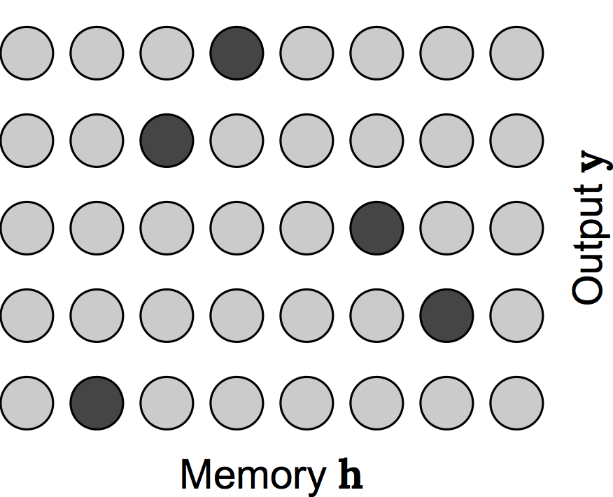
It should be clear that constructing the context vector as a weighted sum of the memory corresponds to computing the expected output of this operation, so we can view an attention mechanism as optimizing this stochastic process in expectation. This allows you to use standard backpropagation to train models which use attention - if our model actually followed this stochastic process at train-time, we'd have to use a gradient estimator like REINFORCE [williams1992]. Also note that for each output timestep the decoder has to make a pass over the entire input sequence. This results in a quadratic complexity, and precludes its use in online settings where output is generated while the input is only partially observed.
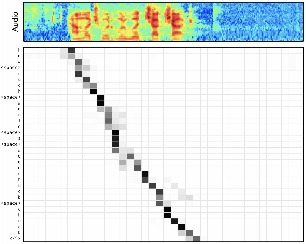
An incredibly useful aspect of attention is that the attention distributions induce a sort of soft input-output alignment which we can visualize. The figure below shows an example from speech recognition, where we are attending over an input speech utterance and producing a sequence of characters as output. Each row in this black and white matrix shows the attention distribution for a given output token. Note that this alignment could be arbitrary, but it's effectively monotonic; that is at a given output timestep the attention probability mass almost never falls before where it was at a previous output timestep. Furthermore although it's a “soft” alignment it's actually pretty peaky, or low-entropy.
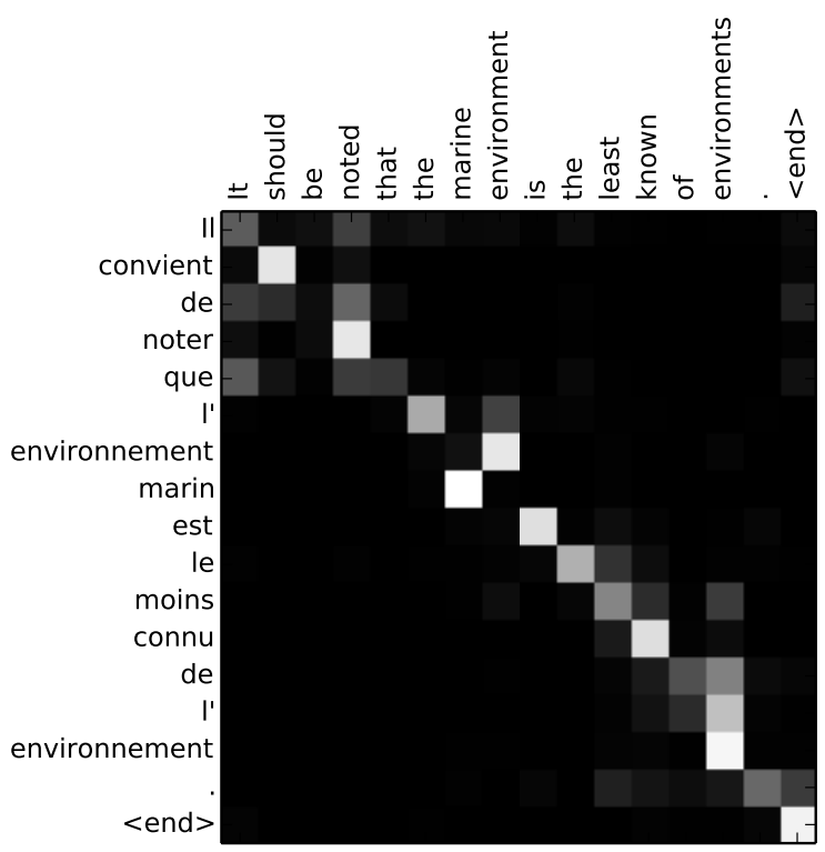
This is true to some extent in other domains as well. Here we are translating an English sentence to a French sentence, and you can again see that the attention distributions are somewhat monotonic and low-entropy. There's some local reordering around the middle, but it's worth noting that the encoder RNN could potentially handle this reordering itself, assuming it's bidirectional.
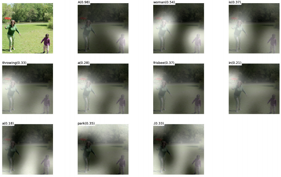
Now of course attention does not always have these properties. Here are the attention “masks” (which are just probability distributions over an image) for an image captioning task. These distributions are definitely smooth, soft, spread-out, and also are certainly not monotonic for any definition of monotonic. So these observations don't always apply.
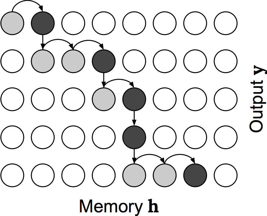
But, let's assume we're working on a task where the alignment is monotonic. Below I'm showing an alternative attention process, which will motivate the monotonic attention mechanism that I'm describing in this blog post. Let's say that at each output timestep, instead of inspecting all entries of the memory independently and choosing one, we start inspecting entries from where we left off at the previous output timestep and explicitly process them in a left-to-right manner. We assign each memory entry a Bernoulli probability which basically denotes “probability of selecting this memory entry to attend to”. As soon as a memory entry is selected, we stop inspecting memory elements and produce an output. For the next output, we start where we left off again. Note that we only make a single pass over the memory when producing the output sequence, so it's linear time. We can also produce outputs as the inputs come in, so it's online. However, it induces a strictly monotonic alignment.
As I mentioned above, actually training a model which has a hard, stochastic attention mechanism like this one precludes backpropagation. One approach for dealing with this would be to train the model with reinforcement learning techniques, and actually there has been some work along these lines. The Reinforcement Learning Neural Turing Machine [zaremba2015] sort of has this mechanism built in, because it makes discrete decisions as to whether to move forward in its input tape or write something to its output tape. More similarly, there has been some work by some of my colleagues at Brain on training a very similar model on speech tasks with REINFORCE, VIMCO, etc. [luo2016] [lawson2017]
But we'll instead follow in the footsteps of soft attention and train models using this monotonic attention mechanism with respect to the expected output of the process I described earlier. In this case, we are still using a soft attention, but the distribution is different. This approach “softly” prevents the model from assigning attention probability before where it attended at a previous timestep by taking into account the attention at the previous timestep.
As a review, here's how the attention distribution is calculated in standard soft attention:
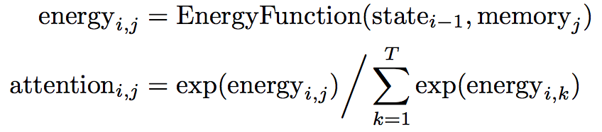
At output timestep \(i\) we first compute an unnormalized “energy” scalar for each entry \(j\) in the memory according to some energy function. The energy is a function of the state at the previous output timestep and the entry in memory we are computing energy for. Then, we just take these energies and normalize them across the memory with the softmax function, shown on the second line.
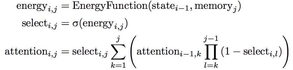
For monotonic attention, we will compute the attention energy in exactly the same way. Then, we'll pass the energies through a logistic sigmoid function, which will give us the “selection probabilities” \(\mathrm{select}_{i, j}\). These probabilities represent the probability that we will select memory item \(j\) and output something, or move on to memory item \(j + 1\). To turn these individual Bernoulli probabilities into a probability distribution over the memory, we use the equation on the bottom:
This is the distribution induced by the monotonic attention process described above. It's a little gnarly, so I've made a little animation to help describe it:
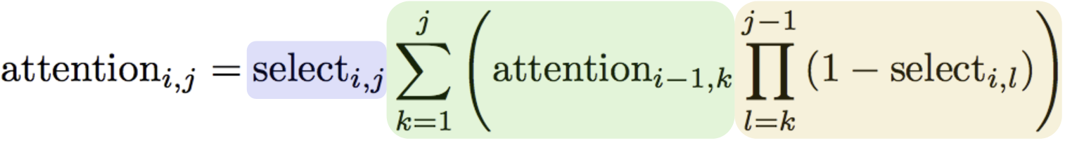
In this animation we are computing the probability of attending to the fourth entry in memory at the third output timestep. We have to consider the possibilities that at the previous (second) output timestep, we attended to the first, second, third, or fourth memory entry, which is shown in green and is what is being animated. For the case that we attended to memory entry \(k\) at the previous timestep, we have to not select any memory entries from \(k\) to to the fourth entry (shown in yellow). Finally, we have to select memory entry \(j\) (shown in blue). So, the green sum is over the four possibilities of where we could have attended at output timestep 2; the yellow product is reflecting that we have to not select memory entries up to the fourth, and then we need to actually attend to the fourth entry which is shown in blue.
One issue with computing the distribution that way is that for each memory-output timestep combination we have to do this sum and product, which gives training-time decoding a cubic complexity if implemented naively. Fortunately, there are lots of shared terms between output timesteps, so we can actually write it as a recurrence relation. This is still bad because it's a recurrence relation, so we have to calculate the terms of the probability distribution sequentially; in other words, we can't parallelize like we do with softmax. Fortunately, we can solve the recurrence relation and express it in terms of cumulative sums and products (which are parallelizable), which gives the following:

Overall, this makes the soft monotonic attention training process have effectively the same speed and complexity as softmax attention while training. I have a full derivation of all of this in Appendix C of the paper, if you're interested.
There's one last thing I haven't addressed, which is that I described this hard monotonic attention process which allows for online and linear-time decoding, but then the training method I described isn't hard, online, or linear-time, because we still compute a probability distribution over the entire memory. But, the idea is that we will train the model in expectation and then use the hard process at test time. In order to do this, we need to ensure the attention distributions are particularly peaky, so the behavior is similar at train and test time. We take a simple and common approach here, where we just add Gaussian noise before the sigmoid activations. This has the effect of making the selection probabilities effectively binary because in order to transmit information through the sigmoid the network needs to make its activation substantially larger than the standard deviation of the Gaussian noise. This is an old trick but there's some nice discussion of it in [foerster2016], Appendix C.
Experiments
To test this approach, we ran experiments on online speech recognition on TIMIT and Wall Street Journal (WSJ), sentence summarization on Gigaword, and machine translation on IWSLT'15 English-to-Vietnamese. Below is the Word Error Rate for the WSJ task.
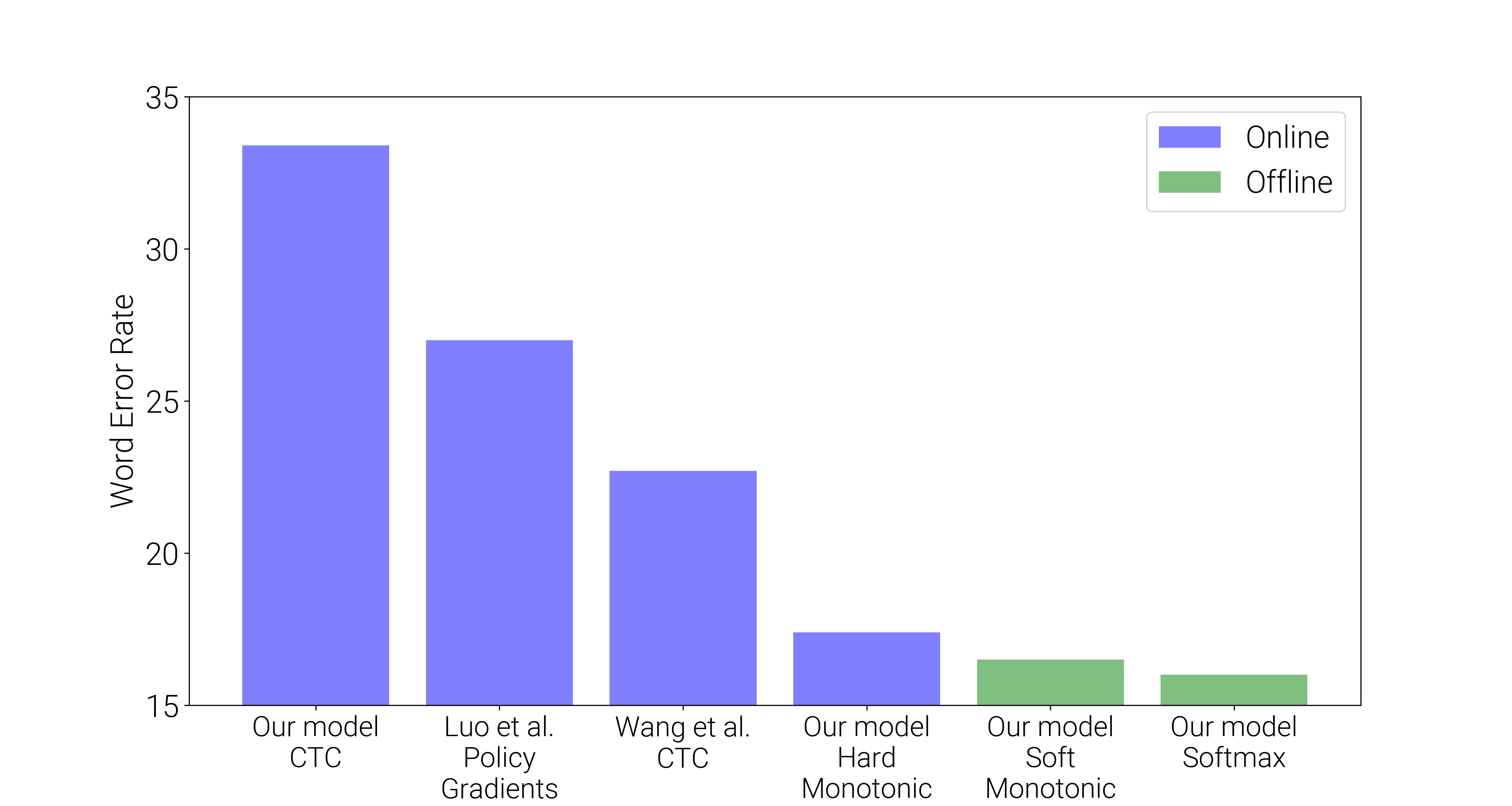
In general, the relative performance of different models was similar to this for all of the experiments. For online WSJ, all the models have unidirectional RNN encoders; the soft monotonic and softmax models were offline because of their attention mechanisms but the other models could all be used online. As is generally the trend, the standard softmax attention model slightly edged out soft monotonic attention (i.e. using the “soft” monotonic attention distribution at test time), which was slightly better than online hard monotonic attention model. I also tested our model with a Connectionist Temporal Classification [graves2006] loss, which did quite a bit worse. The Policy Gradients result is using a similar model to ours, but the model is “hard” at training time too and so a gradient estimator is used. The Wang et al. CTC model is a more realistic representation of the performance of CTC for this task. As I mentioned, in general this was the trend of the results - softmax does best by a small margin, followed by soft monotonic, followed by hard monotonic.
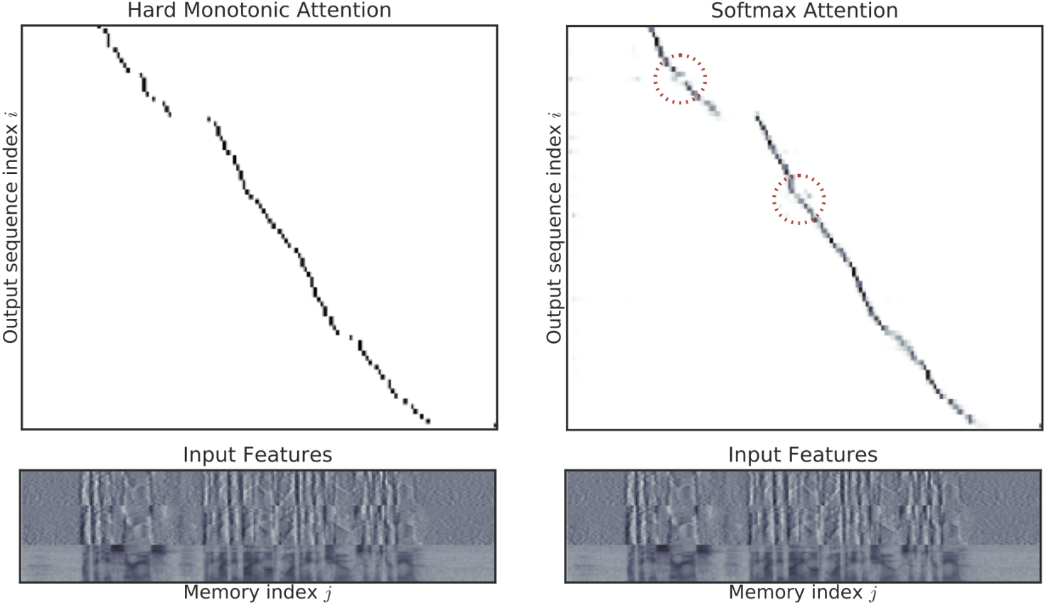
I think it's more informative to look at the alignments the models produced. Below is an example from the WSJ task. In speech recognition, the alignments generally end up looking basically the same. There are some minor differences (which I've circled in red), like the softmax attention spreads out probability and has some minor reordering in places. I'm not sure if this hurts or helps the model.
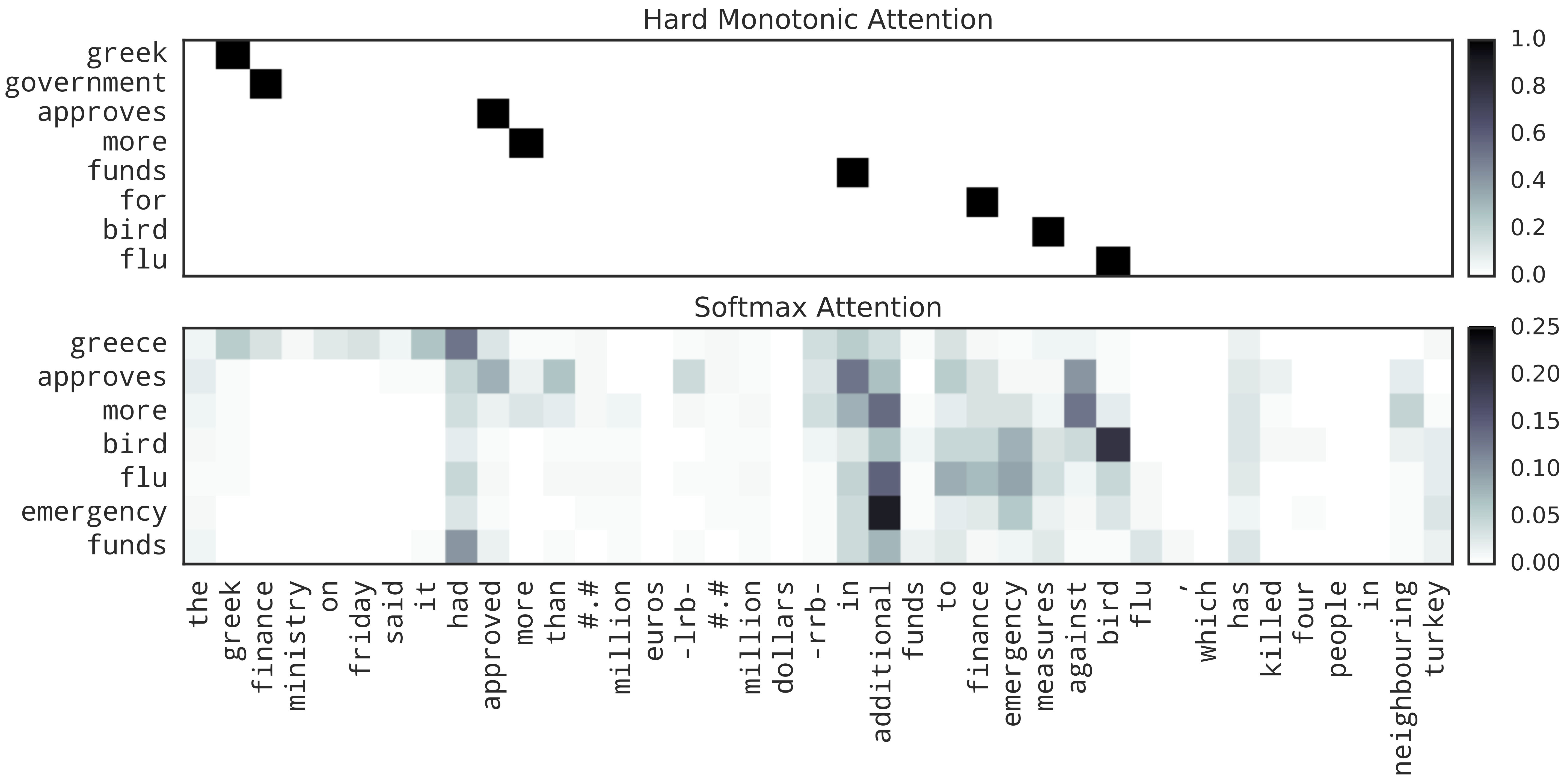
For sentence summarization, we're using a bidirectional encoder, so the encoder can actually do some reordering to the input sequence. We see that in the example below. For hard hard monotonic attention, the first few words are aligned as we expect them to be (greek, finance, approved, more) but the last few words aren't. The model is able to produce a summary which was not monotonically aligned because of the encoder's reordering abilities. You can see that even with softmax attention the alignment isn't obviously what we'd expect it to be, and it actually spreads out attention probability a lot, which again I'm not sure is helpful.
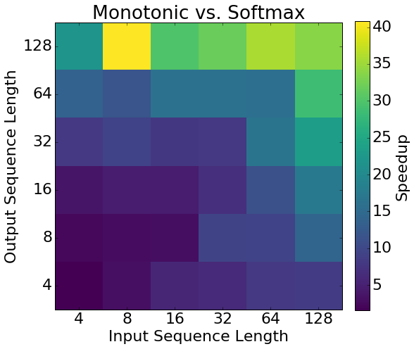
As I've mentioned, one motivation for this approach is that it is potentially much more efficient because the hard monotonic decoder can run in linear time. To test how much faster it can be in practice, we implemented a softmax attention mechanism and a hard monotonic mechanism in C++. We only implemented the attention mechanisms (not the entire sequence-to-sequence model), in order to isolate the difference in speed. The heatmap below shows the speedup for different sequence lengths. We get a speedup of between 4x and 40x. The speedup is particularly strong when the input sequence is short, because the attention basically traverses the entire input sequence quickly after which point we can stop computing context vectors since the attention stays the same.
Code
To help people try this model out, I put an example TensorFlow implementation on GitHub.
The code for the speed benchmark is in the same repository.
I've also added an implementation to tf.contrib.seq2seq, so if you have the latest version of TensorFlow installed you can try it out immediately!
Finally, I added a “practitioner's guide” to Appendix D of the paper, which gives lots of practical tips for getting it to work without trouble.
I'm looking forward to seeing how people apply this approach.